GPU for open-weight models: VRAM, context, and KV-cache

Why VRAM alone is not enough

When choosing a GPU for an open-weight model, people usually start by looking at VRAM. That is useful, but by itself it almost never gives the right answer. A model may fit comfortably in memory, pass a one-request demo, and still start slowing down under normal traffic.

The card’s memory is not used only for weights. Part of it is taken by the model after quantization, part by the KV-cache, which grows as generation continues, and part by service buffers, batching, and the inference engine. That is why an 80 GB card does not automatically mean a comfortable buffer. If the weights already take most of the VRAM, there will be little room left for long conversations and parallel requests.

The biggest factor is context length. A short chat with 10–20 turns usually runs without trouble. A long conversation with history, documents, and system instructions quickly expands the KV-cache, even though the model weights do not change.

The simple takeaway is this: do not choose a GPU because the model fits. Choose it based on three related things — weights, context, and target latency. If you need a first token in 1–2 seconds and stable performance with 20 simultaneous requests, knowing only the VRAM size is not enough. You also need to know how much memory will be left for live sessions and how many tokens per second the card can produce without a queue.

A small example. A team loads a 70B model in quantized form, runs a demo, and sees that everything works. Then they connect it to a support chat where some conversations reach 30–40 messages. Latency jumps sharply. The model did not become heavier. It is just that the KV-cache accumulated, and parallel requests used up the remaining memory.

What data to collect before choosing a GPU

Before choosing hardware, it is more useful to open the logs than the video card catalog. For the calculation, you need not abstract model specs, but the way people actually use your service.

First, collect input length in tokens. Look not only at the average, but also at p95. The average is misleadingly comforting: most requests are short, while the long tail creates the problem. Then look at response length. A bot that usually writes 80 tokens and a bot that regularly generates 600 tokens put very different pressure on the system.

Next, measure load over time. How many requests per second come in during a normal hour, and how many during peak? It is better to use not one lucky day, but at least a few typical weeks. For many teams, the average looks fine, while 10–15 minutes of evening peak break the entire plan.

Another underestimated metric is the number of simultaneously active sessions. Two services can both have 10 RPS and very different GPU load. In one case, those are short independent questions. In the other, there are hundreds of open chats where each conversation history holds memory for KV-cache and cuts parallelism.

Usually, the first working table only needs five rows:

• input length: average, p95, and p99 if available
• response length: average and large outliers
• requests per second: normal hour and peak
• number of simultaneously active sessions
• headroom for growth over at least the next few months

A simple example. For a support desk, the average input is 700 tokens, p95 is 2800, and the average response is 180 tokens. During normal hours, the service handles 4 RPS, at peak 11 RPS, and about 150 dialogs are active at the same time. If you calculate GPU needs using only the average request, the result will almost certainly be too optimistic.

If you do not yet have production logs, use pilot data and immediately leave a reserve. A configuration with less than 20–30% headroom for peak traffic almost always turns out to be too tight sooner than the team expects.

How context changes the calculation

Context length changes the math more than it first appears. Model weights sit in memory almost like a fixed part. KV-cache grows together with the number of tokens. The longer the window, the fewer simultaneous requests the same GPU can handle.

The simplified logic is this: if an 8k-token request needs about 2 GB for KV-cache, then at 32k it needs about 8 GB, and at 128k around 32 GB. The growth is close to linear. That is why choosing a GPU only by VRAM for weights is risky. Very often, memory for context becomes the bottleneck.

Take a simple example. Suppose the weights and service buffers take 48 GB, and the card has only 80 GB total. That leaves 32 GB for live requests. With an 8k window, you can handle about 16 requests at 2 GB each. At 32k, about 4 requests at 8 GB each. At 128k, one long request and, at best, one more in a very tight setup.

That is still a gentle scenario. In a real system, context is almost never just one user message. The memory also includes the system prompt, chat history, app instructions, chunks of documents from RAG, and sometimes a repeated request after a timeout. One retry can easily increase memory pressure if the old session has not yet released its KV-cache.

So you should calculate not by the average conversation, but at minimum by three profiles: a normal request, a long working conversation, and a bad day with long histories, retries, and a spike in parallelism. If the GPU only passes the average scenario, that is not enough for production.

That is why a practical rule is: do not enable a 128k window just in case. It is often cheaper and more stable to keep the main load at 8k or 32k, and enable long context only where it is truly needed.

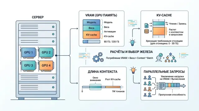
Where the memory goes

It is convenient to split inference memory into three parts: model weights, runtime, and KV-cache. The first part is almost fixed. The second changes moderately. The third follows its own rules and most often breaks the nice calculation on paper.

KV-cache does not grow from model size as such, but from the number of tokens the model has already seen. Every new token adds values for all layers. That is why a long 16k-token dialog uses noticeably more memory than a short 500-token request, even if the model is the same.

As long as there are few sessions, this does not look like a problem. One long session rarely scares anyone. Fifty such sessions quickly hit memory limits before GPU compute becomes the issue. This is especially visible with continuous batching, when the server keeps mixing new requests into ones already in progress and holds many sequences in memory at the same time.

Quantization is a common trap too. It reduces weight memory very well, for example when moving from FP16 to 4-bit. But that does not mean the limit on live conversations will increase just as much. If the engine does not compress KV-cache separately, it often remains in FP16 or BF16. In the end, you save gigabytes on weights, but the limit on active sessions moves much less than expected.

In practice it looks familiar: after quantization, the model fits on one card, the demo works, but as traffic grows, the service still hits OOM on long chats. The problem is not the weights. It is the token history the server keeps for each active conversation.

How to calculate parallelism and latency

Nightly batch processing and live chat put different pressure on a GPU. For a batch job, the total hourly throughput matters. For chat, something else matters more: how many seconds until the first token, and whether the queue grows during the peak.

That is why tokens/s alone is not enough. For an online scenario, you need at least two metrics: time to first token and generation speed after the start. The first one shows how long the user waits. The second one shows whether the answer takes 6 seconds or 20.

Parallelism is also better measured not by average requests per minute, but by short spikes. Suppose you usually get 15 requests per minute, but after a push notification, another 40 arrive within 20 seconds. That kind of jump is what really tests the system. A short spike is survivable. A 10-minute peak breaks the SLA.

For the calculation, a few numbers are enough:

• TTFT for 95% of requests
• full response time for 95% of requests
• average input and output size in tokens
• number of simultaneous requests during the peak interval
• acceptable queue length before SLA is violated

These numbers quickly show how many simultaneous requests the model can handle without a sharp latency increase. If new requests arrive faster than the system can return first tokens, the queue will grow, even if the benchmark shows good tokens/s.

It is useful to check rate limits and canceled responses separately. Limiting by key or client is often better than trying to accept everything at once. That way you keep good latency for most users. Cancellations also affect the calculation: if some people close the response halfway through, the GPU frees up sooner, and the real load ends up lower than the number of started requests suggests.

Step-by-step calculation for your own traffic

It is better to start not with the card choice, but with one working combination: model, precision, and target context length. The same 8B model behaves very differently in FP16, FP8, and INT4. For a rough estimate, memory for weights is calculated simply: multiply the number of parameters by the size of one weight. For an 8B model, that is about 16 GB in FP16, about 8 GB in FP8, and about 4 GB in INT4.

After that, the calculation looks like this.

1. Take the model you actually plan to run and choose the precision. FP16 is usually more predictable, FP8 often gives a good compromise, and INT4 saves a lot of memory, but can reduce quality on harder tasks.

2. Calculate memory for weights and immediately add service overhead. For runtime, the compute graph, and fragmentation, it is reasonable to leave another 15–25% of VRAM. If the card only barely fits the weights, that is not enough for production.

3. Add KV-cache for the required number of sessions. Here, the important thing is not the average, but your real peaks. If the bot keeps 200 sessions with 8–12 thousand tokens, KV-cache can easily become the main limit, even when the model weights fit comfortably.

4. Compare the result with the latency target. A card may fit in memory and still answer too slowly if it has to use a high batch to reach the required throughput. For chat, users notice an extra 300–700 ms very quickly.

5. Then compare the architecture options. One large GPU is usually better for long context and heavy KV-cache: everything stays in one memory pool, without extra exchange between cards. Two smaller cards work if the traffic can easily be split into independent requests and total throughput matters more. For one long session, that option often adds more complexity than value.

If you work through a gateway like AI Router, you still need this calculation. It helps you understand where it is better to keep the open-weight model in-house, and where it makes sense to send rare long requests through an external route.

Example for a support chatbot

Imagine a support desk with 12 new requests per second. The bot answers with an average of 300 tokens and runs on a 32B model with a 32k window. From these numbers alone, the load is clearly high: just to generate replies, you need about 3600 tokens per second.

The memory picture looks like this. In 8-bit form, the 32B model weights take about 32 GB. Several more gigabytes go to service buffers and the inference engine. If you count a full 32k context, KV-cache for such a model can easily reach about 8 GB per active dialog.

With one H100 with 80 GB, the model usually fits, but there is not much comfortable headroom. After loading weights and buffers, about 35–40 GB remains for KV-cache and batching. That means the card can handle only a few simultaneous sessions with the full 32k window. If one response takes at least 3 seconds, then at 12 requests per second there are already about 36 active requests in the system. At that point, you hit both memory and generation latency.

With two L40S cards, the picture is different. The total memory on paper is larger, but it does not add up automatically. For a 32B model, tensor parallelism is usually needed, which means the cards constantly exchange data. Memory is distributed more easily, but latency grows and setup becomes more complex. For a support chatbot, that is an unpleasant compromise: the user cares about a fast first token, and inter-card communication often hurts exactly that.

If real conversations are short, for example 2k–4k tokens instead of 32k, H100 can still make sense for a pilot or a smaller production setup. If long context is needed often, the question is not whether the model fits, but how many simultaneous sessions the KV-cache can handle without a latency spike.

The practical conclusion is simple: one H100 is more convenient as a base node if you need a predictable latency profile and fewer operational complications. Two L40S cards may look cheaper upfront, but they usually bring operational problems faster. For a given traffic pattern, it is more reasonable to think not about one machine, but about several replicas or model routing. Then the 32B model stays for complex conversations, and the bulk of short requests can go to a smaller model.

Where people most often get it wrong

The most common mistake is simple: the team looks only at weight size and thinks the GPU choice is almost done. In practice, that is just the beginning. Memory is consumed by context length, KV-cache, service tokens, batching, and parallel requests. A model may fit on paper and still show sharp latency spikes under normal load.

The second mistake is calculating from the average request. That is convenient, but almost always too optimistic. If the average conversation uses 1800 tokens and 10% of sessions reach 8000, it is that tail that breaks the plan. For support, banking, or telecom, this scenario is normal: the user sends a chat history, a contract, and then asks a clarification question.

The third trap is counting only the user’s text. In a real request, there is the system prompt, history, templates, roles, sometimes chunks from RAG, and service tokens. The actual context is almost always longer than what is visible in the interface.

The fourth mistake is trusting a nice single-stream test. Such a run is useful only for an initial look. In production, parallelism matters: 8, 16, or 32 simultaneous generations behave very differently from one ideal request. With one stream, the card may show great speed, but under real load it can suddenly lose pace because of memory and bandwidth.

And finally, teams often leave no buffer. Today you size for a 4k prompt, and in a month the product asks for 16k, more history, and a second answer-checking stage. A configuration that already looks just barely sufficient today will almost certainly need to be redone.

Final check before buying

Before buying, it is worth doing a short check. Fix one model and one precision. Use p95 and p99 for input and output, not just the average. Look at minute-by-minute peaks, not the daily average load. Then calculate KV-cache for the needed parallelism and add room for growth plus a single-node failure scenario.

In practice, people most often make mistakes in two places: they underestimate long conversation length and overestimate how many parallel sessions the card can handle without a queue. Suppose support usually gets 30 requests per minute and 90 at peak. If the 99th percentile of context length is three times the average, and the system is holding 12–16 active generations in parallel, the card may hit KV-cache limits rather than model weights. Then latency jumps sharply, and the queue builds within a few minutes.

If you are already testing several routes through AI Router, part of this picture can be measured early on real traffic: request length, minute-by-minute peaks, the share of long conversations, and behavior after rate limiting. For teams in Kazakhstan and Central Asia, this is a convenient way to run the same scenarios through one OpenAI-compatible endpoint without rewriting the SDK, code, or prompts.

A good validation result looks boring, and that is normal. You have one chosen model, one precision, real token percentiles, peak load by minute, a KV-cache calculation, 20–30% growth headroom, and a clear plan for a single-node failure. If even one number is missing, it is better to spend another day collecting data than to rebuild the whole setup later.

What to do after the calculation

The paper calculation is important, but the final decision still comes from a live-load test. The table gives you direction. The test quickly shows where the estimate was too bold: context length, number of simultaneous requests, or waiting time in the queue.

Use real prompts or ones that are as close as possible. Do not stop at one average request. Test short conversations, long documents, a spike in user count, and at least one heavy scenario with a large context. During the test, it is enough to watch four metrics: TTFT, tokens/s after start, memory used, and queue time. The combination of these numbers is what matters. For example, tokens/s may look fine, but queue time in the evening can triple. For the user, that is worse than a slightly slower but stable answer.

Then compare two modes: local hosting and API routing. For sensitive data, low latency within the country, or fine-tuned variants, your own setup often makes sense. For rare, heavy, or experimental tasks, access to multiple models via API is often cheaper than buying hardware with a large buffer.

For this kind of check, AI Router can be a useful intermediate step. On airouter.kz, teams can quickly run the same set of scenarios through different frontier models and open-weight options via api.airouter.kz, without changing their familiar SDKs, code, or prompts. That helps show when it is time to build your own GPU cluster and when API routing is enough.

If the test goes well, do not buy the full amount right away. Take one working load profile, leave room in the queue and context, and repeat the measurements with new data in a couple of weeks. That approach is usually cheaper than trying to guess the perfect configuration on the first try.